Intro to Integrals

Riemann Sums

Riemann Sum: a method for approximating area by adding the areas of rectangles.

RRAM- RIGHT Rectangle Approximation Method, using the right endpoint of the graph as the base, and the interval as the height.

LRAM- LEFT Rectangle Approximation Method, using the left endpoint of the graph as the base, and the interval as the height.

MRAM- MIDPOINT Rectangle Approximation Method, using the midpoint of the graph as the base, and the interval as the height. 

TO CALCULATE: interval*(f(x1)+f(x2)+f(x...))

ie. Approximate the area of a region bounded by f(x)=5-x^2 and the x-axis between [0,2]. 

RRAM- .5(f(.5)+f(1)+f(1.5)+f(2))

LRAM- .5(f(0)+f(.5)+f(1)+f(1.5))

MRAM-.5(f(.25)+f(.75)+f(1.25)+f(1.75))

The Trapezoid Rule

Another method of Approximation is the Trapezoid Rule, using trapezoids to find the area under a curve. 

A(trapezoid)= .5h(b1+b2)

Then you just add the areas together. 

A= interval(f(x0) + 2f(x1) + 2(fx2)... + f(xlast))

This is not a Riemann Sum

Integral and Integral Notation

Integral/Integral Notation- The integral is the signed area between the graph of a curve and the x-axis.

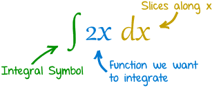
How to write an integral goes as pictured above. When typing the integral into a calculator, you must put the domain in which you are finding the integral. If the domain is [a,b], the b goes at the top of the integral symbol, and the a goes on the bottom as prompted by the calculator. It should look like this. 

To enter an integral into your calculator, press the button that is located next to the open book button. Then chose the prompt highlighted below, and type the equation as shown above.

Concavity and the Second Derivative Test

Concavity and the 2nd Derivative Test

New Vocabulary:

• Inflection Point: 
• Point where the concavity of the graph changes sign.
• Found where f''=0 or undefined
• Concavity
• The curve or shape of a line
• f''>0 the function is concave up (smily face)
• f''<0 the function is concave down (frowny face)

Example:

Determine the open interval on which f(x) is concave up and/or concave down, and all inflection points. f(x)=6 / (x^2+3)

ONE: Find first and second derivative

f(x)=6/(x^2+3)                        **Rearrange function so it is easier to take the first derivative
      =6(x^2+3)^-1

f'(x)= -6 (x^2+3)^-2 (2x)        **Take first derivative and simplify
       = -12x / (x^2+3)^2

f''(x)= [(x^2+3)^2 (-12) - (-12x) (2) (x^2+3) (2x)] / (x^2+3)^4         **Take the derivative
       = (x^2+3) (-12(x^2+3) + 48x^2) / (x^2+3)^4          **Factor out (x^2+3) then cancel with bottom
       = -12 [(x^2+3) - 4x^2] / (x^2 +3)^3                                            ** Factor out -12
       = -12 (-3x^2+3) / (x^2 +3)^3                                                       ** Simply top
       = 36 (x^2-1) / (x^2+3)^3                                          ** Factor out -3 and multiply with -12

TWO: f''(x) = 0 or undefined

f''(x)= 36 (x^2-1) / (x^2+3)^3

36 (x^2-1) = 0                         ** Set top equal to zero to find POSSIBLE inflection points
x= -1, 1                                   ** POSSIBLE Inflection points

Bottom is never undefined! (x^2 +3)^3 can never equal zero

THREE: Plug inflection points into original to find the y-values to the point (use calc.)

f(1) = 6 / (1^2 + 3)^2 = 3/2
f(-1) = 6 / (-1^2 +3)^2 = 3/2

FOUR: Create a number line to test the inflection points

1. Test x= -2, 0, 1 in f''(x) to see if positive or negative (shown below test number)
2. Where f''(x)>0 the function is concave up 
3. Where f''(x)<0 the function is concave down

FIVE: Answer the question

Concave up: (1, infinity) and (- infinity, -1)
Concave down: (-1,1)
Inflection Points: (1, 3/2) and (-1, 3/2)

The First Derivative Test

                                                                                                                 Briya Kirksey
We have now started to learn about the derivative application #3 which is Curve Sketching. You can find this section in our calculus book labeled as "Connecting the Graphs of f ', f '', and f''' ". The first part of this section is "The First Derivative Test".

                           The First Derivative Test 

     What are we looking for?

• We are taking a functions equation and determining where it is  increasing and/ or decreasing, and its relative extrema (relative maximum/minimum) on its graph. 

   

  How do we do this?

  1.   Take the derivative of the given function (if its not already given). 
  2.   Set the derivative equal to zero. Why? - Because that is where the slopes of the functions graph changes signs (positive to negative or vise versa). The values we get by doing this is what we know as critical points. 
  3. Make an x-axis number line labeling all of the critical points on it. 
  4. Choose numbers on the number before, after, and in between the critical points, known as testing points. Example: If critical points are x= -1, 0, 3 , then my testing points could be x= -1.5, -.5, 2, 4. 
  5. Plug each of the testing points into the derivative. Why?- To determine the behavior of the functions graph in between its critical points. 
  6. The answers produced by doing step number 5 will give you the x intervals in which the graph is increasing/decreasing and which x values there may be a max/min.  

                 Tip: 

  • When plugging in testing points into a functions derivative, pay attention to the values sign to make it easier in determining whether the slope will be positive or negative.
   Example:  y' = x (x-3)^2   testing point : -1
  
   Without doing any math, one can already tell that the slope will end up being negative. The value in the parenthesis is -4, but the fact that it is then squared makes it positive. However the x value  (-1) being multiplied to the positive value makes the slope  negative.   

  Concavity : Refers to the way Graphs look

  This is the worksheet and notes used to learn about Concavity. Concave up= a u-shape facing up. Concave down= u -shape facing downward. Inflation point= point on graph where cure changes; where y '' = 0. 

   

  

  
  

     

   

Existence Theorems

This week, we learned about the first application of derivatives: Existence Theorems. Basically, the theorems state that a certain point exists if it meets some criteria. Here are the four types of Existence Theorems we learned about.

1. Intermediate Value Theorem (IVT)
     - if a function f(x) is continuous on a closed interval [a,b]
     - and k (a y-value) is any value between f(a) and f(b)
     - then there is at least one number "c" (an x-value) in [a,b] such that f(c)= k

An example question: if f(x)= x^3+2x-1 is there a value on the interval [0,1] where c is 0?
     -First, determine if the function is continuous on the interval: in this case, it is
     -Second, find the values of f(0) and f(1)
          -      f(0)= -1      f(1)= 2
     -Since -1<0<2, a "c" exists on the interval such that f(c)= 0
     -To find this, we simply set the equation equal to 0.
          -      x^3+2x-1=0    if you solve this, and plug it into the calculator, c=.453   

2. Extreme Value Theorem (EVT)
     -if f(x) is continuous on the interval [a,b]
     -then f(x) is guaranteed to have an absolute minimum and an absolute maximum on the interval

An Extreme Value can happen at two places: endpoints and critical points (where the derivative is equal to 0 or is undefined)

An Example Question: Can you apply EVT to the equation x^-1 +4x on the interval [-4, -.25]? If so, what are the absolute maximum and minimum?
     -First, determine if the function is continuous on the interval.
          - x is not defined at 0, but this is not in the interval, so it doesn't matter
     -Second, evaluate f(-4) and f(-.25) to find possible points for extreme values
          - f(-4)= -16.25     f(-.25)= -5
     -Third, find the critical points by finding f'(x) and determining where the derivative= 0 or und.
          - f'(x)= -1    +4
                      x^2   
          - this is undefined at x=0, but isn't on the interval, so it doesn't matter
          - f'(x) equals zero at x= .5 or -.5 (however, .5 is not on our interval so it doesn't matter)
     -Fourth, evaluate f(x) at critical points
          - f(-.5)= -4
     -Finally, we can determine where the absolute maxes and mins are. In this situation, the maximum is -4 at x= -.5   and the minimum is -16.25 at x= -4

3. Mean Value Theorem (MVT)
     - if f(x) is continuous on [a,b] AND
     - if f(x) is differentiable on (a,b)
     - then there exists a number "c" in (a,b) such that
                 f'(c)= f(b)-f(a)
                              b-a

An Example Question: Is MVT applicable to the equation x+1/x on the interval [.5, 2]? If so, find the value of c.                                                                            
     - First, determine if the function is continuous and differentiable on the interval. In this case, it is, so MVT applies.
     - Second, evaluate f(.5) and f(2)
            -  f(.5)= 3    f(2)= 1.5
     - Third, plug these values into f(b)-f(a)
                                                          b-a
               In this case, it will simplify to -1
     - Fourth, find f'(x) and set it equal to -1.
          -   -1= -1  
                     x^2
          - x= 1, -1 (however, -1 is not on the interval, so we disregard this.) c=1

4. Rolle's Theorem (RT)
     - if f(x) is continuous on [a,b] AND
     - f(x) is differentiable on (a,b) AND
     - f(a)=f(b)
     - then there exists some number "c" on the interval (a,b) such that f'(c)=0

An Example Question: Is RT applicable to the equation f(x)=sin2x on the interval [π/2, 3π/8]? If so, find the value of c.
     - First, determine if the function is continuous and differentiable on the interval.
 In this case, it is.
     - Second, determine what f(π/2) is and f(3π/8) is.
          - f(π/2)= √2/2  f(3π/8)= √2/2 so yes, they are equal and MVT applies.
     - Third, find f'(x) and set it equal to 0 to find c.
          - f'(x)= 2cos2x 
               - 2cos2x= 0           x=π/4, 3π/4 (however, 3π/4 is not on the interval, so it is not included. c=π/4


That is what we did in class this week! Existence Theorems are so fun just like calculus yay!
 

L'Hopital's Rule- Sean Dandeneau

L’Hopital’s Rule

We recently learned how to use L’Hopital’s rule when we must do so. This situation appears whenever we try to evaluate limits that produce indeterminate forms when we try direct substitution.

To use L’Hopital’s rule, you must find the derivatives of the numerator and the denominator. Once this is found, you plug in c for  x and solve for the limit as x->c.

Lim of f(x)/g(x) as x->c = lim of f’(x)/g’(x) as x->c = lim of f’’(x)/g’’(x) as x->c

Lim 1-cos(x)/x as x->0

= 0/0

    So we must use L’Hopital’s Rule…

Lim 0-(-sin(x))/1 as x->0

= lim sin(x) as x->0

= sin(0)

= 0

When doing L’Hopital’s Rule, we must keep in mind that all derivative rules apply. We can find as many derivatives as we need to in order to solve for the limit at c.

Another example:

f(x)=lnx^5/x

Lim x->infinity lnx^5/x

    = lim x->infinity 5lnx/x

    = lim x->infinity (5/x)/1

    = lim x-> infinity 5/x

    = lim x-> infinity 0/1

    = 0

Continuity and Discontinuity

Over the weekend, our homework was to complete a survey evaluating limits through the topic of roads and bridges. On Monday, we began our discussion on continuity by thinking in these roads and bridges terms:

Continuity- a function f(x) is continuous at x=a if

1. the roads meet
2. there is a bridge
3. the roads meet at the bridge

After conceptually understanding what continuity is, we decided to translate this definition into calculus lingo.

Continuity- a function f(x) is continuous at x=a if

1. the limit of x as it approaches a exists
2. f(a) exists
3. the limit of x as it approaches a is equal to f(a)

In other words

• If you can draw it without lifting your pencil, it’s continuous.
• f(x) is continuous at x=a if
• the limit from the left equals the limit from the right (or the roads come to the same spot)
• a y-value exists at x=a (bridge exists; there isn’t a hole or asymptote there)
• the y-value, the limit from the left, and the limit from the right are all the same number

Discontinuity

• A function has a point of discontinuity at x=a if it fails one or more of the four criteria listed below

The Four Types of Discontinuities and How to Find Them:

1. Removable
1. Piecewise function
2. Hole (a factor cancels)
2. Jumps
1. Absolute value division function
2. Greatest integer function
3. Piecewise function
3. Infinite
1. y=tan(x) (infinite discontinuities at odd integers of pi/2)
2. Reciprocal (vertical asymptote- cannot cancel an x in the denominator)
4. Restricted
1. Square root (continuous for all x-values in its domain, but not outside its domain)
2. Logarithms (only continuous for x>0, unless it is transformed)

The worksheet for discontinuity:

Based on the definition of continuity and the four types of discontinuity, we were able to solve the following problems in class:

To find a value that makes a function continuous, plug in the the boundary (in this case, the boundary is 1) into the x of each part of the piecewise function and solve. Then, set up the answers from each part of the piecewise function and save for a, as shown above. 

Here are answers to the homework problems!

Differentiability

Differentiability: f(x) is not differentiable at x=a (f’(x) does not exist) when f’(x) is not continuous at x=a.

For example:

The Four Ways a Function can Fail to be Differentiable at x=a:

1. A corner
1. Different one sided derivatives causes the graph to jump (ex. absolute value graph)
2. A vertical tangent
1. One-sided derivatives go toward infinity (ex. y=x^⅓)
3. A cusp
1. One-sided derivatives go toward opposite infinities (one toward positive infinity and the other toward negative infinity)
4. Any type of discontinuity
1. Any of the four types of discontinuity explained in the previous section!

The worksheet for differentiability:

Remember:

• Continuity does not imply differentiability, but
• Differentiability does imply continuity.

In other words:

• f’(c)=lim x as it approaches c [f(x)-f(c)]/(x-c) must exist if f is differentiable at x=c

Based on these notes of differentiability, we were able to complete the following in class problems:

To make it differentiable, you find the derivative of the top part of the piecewise function and the derivative of the bottom of the piecewise function, set them equal to one another, and then solve. In this case, you also had to make it continuous, which is explained in a problem above. 

Here are the homework answers!

Reminder

Don’t forget to study for the assessment on tuesday!

Blog for November 4

Overview:
This week we began learning about limits. We had seen limits before, at the beginning of the derivatives unit. The limit definition of the derivative of a function at a point helped us find the slope of the tangent line at x=c. The limit definition of the derivative of a whole function was used to find the slope of a secant line between any point on f(x) and another point that is h units away from it.
As we move away from the topic of derivatives, we focused on limits as x approaches any point in a function.

Graphical Approach
There are three main approaches to limits. We began with the graphical approach. This entails using graphs to find the limit at a point.


We were asked to find the limits from the left and right of each point pictured, as well as the actual limit for each value.


We learned that the limit does not exist if the limits approaching from the left and right sides are different from each other. The limit also does not exist if either of these values is infinity or negative infinity. In other words...


We then did some practice finding limits using graphs.



Numerical Approach
The next approach is the numerical approach. For this approach, we use a table to determine the limits approaching a point from the left and right. As the value gets closer to x, the limit gets closer to what it should be. For example:

In this example, the limits on either side seem to be approaching the same number, .333. This means the limit as x is approaching 2 is .333. If the limits on  either side are not approaching the same number, or they are approaching infinity or negative infinity, the limit does not exist.


Analytical Approach
The last approach is the analytical approach. This is when you use direct substitution to find the limit. You plug in the value, c, into the function, f(x). For normal functions, if the limit as x approaches c exists, it should be f(c).
 
In the last example, the limit ends up being 0/0. This means that there is a hole in the graph at this point.



We were also introduced to the properties of limits in class, which are listed below.


The last topic we covered this week was limits at infinity. This involves plugging infinity into functions as the x-value,  which would result in finding the end behavior of functions. To find the end behavior or a horizontal asymptote, you need to find the limit as x approaches both infinity and negative infinity.
 

Reminder: Monday's class will be a review for our quiz on Thursday.