Properties of Integrals

Properties of Integrals:

Different Properties of Integrals can be used to evaluate certain integral equations.

To evaluate an integral:

1. f(x) must be defined

2. The function must be continuous on the interval

Adding/Subtracting Integrals:

 Integrals with an interval of 0:

 Multiplying Integrals by a constant:

 Adding Integrals of adjacent intervals:

 Negative Integrals:

Example from textbook (pg. 290 #2):

a. (-2) ∫f(x)dx = (-2)(-1) = 2

b. ∫f(x)dx + ∫h(x)dx = 5+4 = 9

c. ∫[(2)∫f(x) - (-3)∫h(x)]dx

    (2)∫f(x)dx - (-3)∫h(x)dx = (2)(5)-(-3)(4) = 10+12 = 22

d. ∫f(x)dx = 1

e. (from 1 to 9)∫f(x)dx + (from 7 to 1)∫f(x)dx =  (from 7 to 9)∫f(x)dx =  

    -1 + -∫f(x)dx = 5

    5 +1 = 6

    -6 = (from 1 to 7)∫f(x)dx

f.  ∫h(x)dx - ∫f(x)dx = 4-5 = -1

*keep in mind that the intervals must be the same as what you are evaluating for as I could not type and show that here

Derivatives of Inverse Functions

Inverse Functions:

Inverse functions can be written as f^(-1)(x) and they occur when the y and x values of a function are switched so that the graph flips over dotted line in the example below.



Finding the Derivative of an Inverse Function:

The derivative of an inverse function is the same as the reciprocal of the derivative of the original function when the x value of the inverse function is equal to the y value of the function. In other words, to find the derivative of the function you must:

1. Find the x value of the original function so that the y value original function is equal to the x value of the inverse function.
2. Find the derivative of the original function when x is equal to the x value you found in step 1.
3. Find the derivative of the inverse function by finding the reciprocal of the answer from step 2. (In other words flip the fraction, but remember that the sign does not change)

Example:
Find (f^-1)'(3) when f(x) = -x^2+5

3 = x+5
5-3 = x
2 = x
f'(x) = -2x^1+0 = -2x
f'(2) = -2(2) = -4
(f^-1)'(3) = -1/4

Sometime you are given a chart instead of an equation.

Example:

Find (g^-1)'(3)

3 = g(x)
x = 4
g'(4) = 1/2
(g^-1)'(3) = 2

Intro to Integrals

Riemann Sums

Riemann Sum: a method for approximating area by adding the areas of rectangles.

RRAM- RIGHT Rectangle Approximation Method, using the right endpoint of the graph as the base, and the interval as the height.

LRAM- LEFT Rectangle Approximation Method, using the left endpoint of the graph as the base, and the interval as the height.

MRAM- MIDPOINT Rectangle Approximation Method, using the midpoint of the graph as the base, and the interval as the height. 

TO CALCULATE: interval*(f(x1)+f(x2)+f(x...))

ie. Approximate the area of a region bounded by f(x)=5-x^2 and the x-axis between [0,2]. 

RRAM- .5(f(.5)+f(1)+f(1.5)+f(2))

LRAM- .5(f(0)+f(.5)+f(1)+f(1.5))

MRAM-.5(f(.25)+f(.75)+f(1.25)+f(1.75))

The Trapezoid Rule

Another method of Approximation is the Trapezoid Rule, using trapezoids to find the area under a curve. 

A(trapezoid)= .5h(b1+b2)

Then you just add the areas together. 

A= interval(f(x0) + 2f(x1) + 2(fx2)... + f(xlast))

This is not a Riemann Sum

Integral and Integral Notation

Integral/Integral Notation- The integral is the signed area between the graph of a curve and the x-axis.

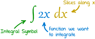
How to write an integral goes as pictured above. When typing the integral into a calculator, you must put the domain in which you are finding the integral. If the domain is [a,b], the b goes at the top of the integral symbol, and the a goes on the bottom as prompted by the calculator. It should look like this. 

To enter an integral into your calculator, press the button that is located next to the open book button. Then chose the prompt highlighted below, and type the equation as shown above.

Concavity and the Second Derivative Test

Concavity and the 2nd Derivative Test

New Vocabulary:

• Inflection Point: 
• Point where the concavity of the graph changes sign.
• Found where f''=0 or undefined
• Concavity
• The curve or shape of a line
• f''>0 the function is concave up (smily face)
• f''<0 the function is concave down (frowny face)

Example:

Determine the open interval on which f(x) is concave up and/or concave down, and all inflection points. f(x)=6 / (x^2+3)

ONE: Find first and second derivative

f(x)=6/(x^2+3)                        **Rearrange function so it is easier to take the first derivative
      =6(x^2+3)^-1

f'(x)= -6 (x^2+3)^-2 (2x)        **Take first derivative and simplify
       = -12x / (x^2+3)^2

f''(x)= [(x^2+3)^2 (-12) - (-12x) (2) (x^2+3) (2x)] / (x^2+3)^4         **Take the derivative
       = (x^2+3) (-12(x^2+3) + 48x^2) / (x^2+3)^4          **Factor out (x^2+3) then cancel with bottom
       = -12 [(x^2+3) - 4x^2] / (x^2 +3)^3                                            ** Factor out -12
       = -12 (-3x^2+3) / (x^2 +3)^3                                                       ** Simply top
       = 36 (x^2-1) / (x^2+3)^3                                          ** Factor out -3 and multiply with -12

TWO: f''(x) = 0 or undefined

f''(x)= 36 (x^2-1) / (x^2+3)^3

36 (x^2-1) = 0                         ** Set top equal to zero to find POSSIBLE inflection points
x= -1, 1                                   ** POSSIBLE Inflection points

Bottom is never undefined! (x^2 +3)^3 can never equal zero

THREE: Plug inflection points into original to find the y-values to the point (use calc.)

f(1) = 6 / (1^2 + 3)^2 = 3/2
f(-1) = 6 / (-1^2 +3)^2 = 3/2

FOUR: Create a number line to test the inflection points

1. Test x= -2, 0, 1 in f''(x) to see if positive or negative (shown below test number)
2. Where f''(x)>0 the function is concave up 
3. Where f''(x)<0 the function is concave down

FIVE: Answer the question

Concave up: (1, infinity) and (- infinity, -1)
Concave down: (-1,1)
Inflection Points: (1, 3/2) and (-1, 3/2)

The First Derivative Test

                                                                                                                 Briya Kirksey
We have now started to learn about the derivative application #3 which is Curve Sketching. You can find this section in our calculus book labeled as "Connecting the Graphs of f ', f '', and f''' ". The first part of this section is "The First Derivative Test".

                           The First Derivative Test 

     What are we looking for?

• We are taking a functions equation and determining where it is  increasing and/ or decreasing, and its relative extrema (relative maximum/minimum) on its graph. 

   

  How do we do this?

  1.   Take the derivative of the given function (if its not already given). 
  2.   Set the derivative equal to zero. Why? - Because that is where the slopes of the functions graph changes signs (positive to negative or vise versa). The values we get by doing this is what we know as critical points. 
  3. Make an x-axis number line labeling all of the critical points on it. 
  4. Choose numbers on the number before, after, and in between the critical points, known as testing points. Example: If critical points are x= -1, 0, 3 , then my testing points could be x= -1.5, -.5, 2, 4. 
  5. Plug each of the testing points into the derivative. Why?- To determine the behavior of the functions graph in between its critical points. 
  6. The answers produced by doing step number 5 will give you the x intervals in which the graph is increasing/decreasing and which x values there may be a max/min.  

                 Tip: 

  • When plugging in testing points into a functions derivative, pay attention to the values sign to make it easier in determining whether the slope will be positive or negative.
   Example:  y' = x (x-3)^2   testing point : -1
  
   Without doing any math, one can already tell that the slope will end up being negative. The value in the parenthesis is -4, but the fact that it is then squared makes it positive. However the x value  (-1) being multiplied to the positive value makes the slope  negative.   

  Concavity : Refers to the way Graphs look

  This is the worksheet and notes used to learn about Concavity. Concave up= a u-shape facing up. Concave down= u -shape facing downward. Inflation point= point on graph where cure changes; where y '' = 0. 

   

  

  
  

     

   

Existence Theorems

This week, we learned about the first application of derivatives: Existence Theorems. Basically, the theorems state that a certain point exists if it meets some criteria. Here are the four types of Existence Theorems we learned about.

1. Intermediate Value Theorem (IVT)
     - if a function f(x) is continuous on a closed interval [a,b]
     - and k (a y-value) is any value between f(a) and f(b)
     - then there is at least one number "c" (an x-value) in [a,b] such that f(c)= k

An example question: if f(x)= x^3+2x-1 is there a value on the interval [0,1] where c is 0?
     -First, determine if the function is continuous on the interval: in this case, it is
     -Second, find the values of f(0) and f(1)
          -      f(0)= -1      f(1)= 2
     -Since -1<0<2, a "c" exists on the interval such that f(c)= 0
     -To find this, we simply set the equation equal to 0.
          -      x^3+2x-1=0    if you solve this, and plug it into the calculator, c=.453   

2. Extreme Value Theorem (EVT)
     -if f(x) is continuous on the interval [a,b]
     -then f(x) is guaranteed to have an absolute minimum and an absolute maximum on the interval

An Extreme Value can happen at two places: endpoints and critical points (where the derivative is equal to 0 or is undefined)

An Example Question: Can you apply EVT to the equation x^-1 +4x on the interval [-4, -.25]? If so, what are the absolute maximum and minimum?
     -First, determine if the function is continuous on the interval.
          - x is not defined at 0, but this is not in the interval, so it doesn't matter
     -Second, evaluate f(-4) and f(-.25) to find possible points for extreme values
          - f(-4)= -16.25     f(-.25)= -5
     -Third, find the critical points by finding f'(x) and determining where the derivative= 0 or und.
          - f'(x)= -1    +4
                      x^2   
          - this is undefined at x=0, but isn't on the interval, so it doesn't matter
          - f'(x) equals zero at x= .5 or -.5 (however, .5 is not on our interval so it doesn't matter)
     -Fourth, evaluate f(x) at critical points
          - f(-.5)= -4
     -Finally, we can determine where the absolute maxes and mins are. In this situation, the maximum is -4 at x= -.5   and the minimum is -16.25 at x= -4

3. Mean Value Theorem (MVT)
     - if f(x) is continuous on [a,b] AND
     - if f(x) is differentiable on (a,b)
     - then there exists a number "c" in (a,b) such that
                 f'(c)= f(b)-f(a)
                              b-a

An Example Question: Is MVT applicable to the equation x+1/x on the interval [.5, 2]? If so, find the value of c.                                                                            
     - First, determine if the function is continuous and differentiable on the interval. In this case, it is, so MVT applies.
     - Second, evaluate f(.5) and f(2)
            -  f(.5)= 3    f(2)= 1.5
     - Third, plug these values into f(b)-f(a)
                                                          b-a
               In this case, it will simplify to -1
     - Fourth, find f'(x) and set it equal to -1.
          -   -1= -1  
                     x^2
          - x= 1, -1 (however, -1 is not on the interval, so we disregard this.) c=1

4. Rolle's Theorem (RT)
     - if f(x) is continuous on [a,b] AND
     - f(x) is differentiable on (a,b) AND
     - f(a)=f(b)
     - then there exists some number "c" on the interval (a,b) such that f'(c)=0

An Example Question: Is RT applicable to the equation f(x)=sin2x on the interval [π/2, 3π/8]? If so, find the value of c.
     - First, determine if the function is continuous and differentiable on the interval.
 In this case, it is.
     - Second, determine what f(π/2) is and f(3π/8) is.
          - f(π/2)= √2/2  f(3π/8)= √2/2 so yes, they are equal and MVT applies.
     - Third, find f'(x) and set it equal to 0 to find c.
          - f'(x)= 2cos2x 
               - 2cos2x= 0           x=π/4, 3π/4 (however, 3π/4 is not on the interval, so it is not included. c=π/4


That is what we did in class this week! Existence Theorems are so fun just like calculus yay!
 

L'Hopital's Rule- Sean Dandeneau

L’Hopital’s Rule

We recently learned how to use L’Hopital’s rule when we must do so. This situation appears whenever we try to evaluate limits that produce indeterminate forms when we try direct substitution.

To use L’Hopital’s rule, you must find the derivatives of the numerator and the denominator. Once this is found, you plug in c for  x and solve for the limit as x->c.

Lim of f(x)/g(x) as x->c = lim of f’(x)/g’(x) as x->c = lim of f’’(x)/g’’(x) as x->c

Lim 1-cos(x)/x as x->0

= 0/0

    So we must use L’Hopital’s Rule…

Lim 0-(-sin(x))/1 as x->0

= lim sin(x) as x->0

= sin(0)

= 0

When doing L’Hopital’s Rule, we must keep in mind that all derivative rules apply. We can find as many derivatives as we need to in order to solve for the limit at c.

Another example:

f(x)=lnx^5/x

Lim x->infinity lnx^5/x

    = lim x->infinity 5lnx/x

    = lim x->infinity (5/x)/1

    = lim x-> infinity 5/x

    = lim x-> infinity 0/1

    = 0